Learning Satistics via Sabermetrics
by Alex Nelson, 21 June 2015
Abstract: As a playground for statistical thinking, we examine baseball data. Very crude and basic statistical heuristics are introduced, the mean & standard deviation discussed, and the linear regression heuristically motivated. We make some embarrassingly wrong predictions.
We assume some familiarity with probability. Those who want to learn more about probability are free to read my notes.
Contents
Introduction
I needed to learn statistics, so I thought I would try to learn it through applying the tools to baseball (“sabermetrics” is the technical term for quantitative baseball). If you do not know the rules of the game, there’s a 8 minute YouTube Video summarizing it.
Generally, “baseball season” starts towards the end of March, and ends at the beginning of October.
The game seems pretty simple, so how hard can it be to quantitatively describe it? There are:
- 41 batting statistics
- 7 base run statistics
- 50 pitching statistics
- 12 fielding statistics
- 3 “overall player value” statistics, and
- 4 statistics associated to each game
…for a grand total of 117 statistics to juggle around. How can we tell which ones are valuable and which ones are junk?
Already, this appears quite daunting: what do we even want to do with our 117 statistics?
Step 0: Formulate a problem we wish to solve with our given data. (End of Step 0)
Problem Statement
Find a function which, given two baseball teams who will play each other, will produce the winner of the game.
Extra Credit. Predict the end score for the game.
Basic Solution. The basic idea would be to predict the “runs scored” variable (R) for each team. Whichever one is higher naturally indicates the winner. (In the argot of statistics, the number of runs for a given game will be the response variable — i.e., we want to “model”, i.e. construct a function, R(…) which will approximate the number of runs by the end of the game.)
Getting Setup
I did most of the difficult work already, and one just has to follow the
instructions in the documentation for the project.
Checkout v0.1.0 for the relevant code.
First Steps
“Great, we have a huge database full of data, what do I do?” Well, in general, we usually want to examine the variables and identify them as either categorical, continuous, or ordinal (think of this as an ordered statistic with finite values, like on surveys where you can judge some service as “Best”, “Good”, “Neutral”, “Bad”, “Horrible”).
Step 1: Examine the data, specifically the data related to the question we posed in step 0. (End of Step 1)
This includes examining the average value for the relevant signals. We will soon find out, as Nate Silver pointed out, “The average is still the most useful statistical tool ever invented.”
For us, lets consider examining a few values. We’re interested in the runs in a game, and homeruns are related to the number of runs so lets look at those too. Lets see the raw data for the past 10 years:
sabermetrics.team> (def t1 (since 2005))
sabermetrics.team> (reduce + (map :games-played t1))
43736
sabermetrics.team> (reduce + (map :hits t1))
388118
sabermetrics.team> (reduce + (map :runs t1))
195074
sabermetrics.team> (reduce + (map :homeruns t1))
43209
Remark on Double Counting. Note that a baseball game involves two teams, so if we just add up all the games each team has been in…we’ll double count the number of games. Just bear this in mind when performing the statistical analysis. (End of Remark)
So, it’s interesting:
- the ratio of runs to hits is approximately roughly 50.26%,
- an average of 8.92 runs per game,
- 17.75 hits per game on average,
- the ratio of home runs to runs is approximately 20.15%, or 1/5,
- whereas there is roughly 2 home run per game on average (well, 1.9759 home runs per game, but still!).
What do these statistics look like for the past 5 years or so?
We have the following table summary:
| Year | Runs per Game | Homeruns Per Game | Homeruns to Runs Ratio |
|---|---|---|---|
| 2010 | 8.768724 | 1.8983539 | 0.21649146 |
| 2011 | 8.566488 | 1.8740222 | 0.21876201 |
| 2012 | 8.648972 | 2.0304527 | 0.23476234 |
| 2013 | 8.331963 | 1.917318 | 0.23011602 |
| 2014 | 8.132099 | 1.7226337 | 0.21183139 |
Home runs per game fluctuating “a bit”, runs per game “roughly steady”, and the ratio of home runs to runs “steady-ish”.
Observations. (1) We should probably formalize a notion of “fluctuating a bit”, versus “steady-ish”. In this manner, we can rigorously say “This signal is more x-times more steady than that one.” (2) Analyzing these ratios year-by-year is tiresome and error-prone (saying “Yep, that looks good enough” is error-prone). We need some way to get the data with a cursory glance. (End of Observations)
Variance
We can determine the magnitude of fluctuation by using
“Variance”. There is actually quite a bit of subtlety to this
notion, but it is surprisingly simple: it measures “how far off” the
mean is from the sample values. Consider the sample
[5, 3, 1, 3, 5]. We see its average is 17/5=3.4. We can plot these
data points, the mean as a horizontal line, and red arrows from the data
points to the mean:
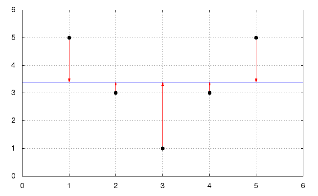
The average for the sum of the squares of the lengths of the red line segments is the variance, its square-root is the standard deviation. The labels on the x-axis just indicates which element of our list we’re examining. The average square-distance to the mean, is our intuitive picture of the variance. (Hey, the average is used to figure out how much a data set varies, pretty nifty.)
Definition. Given a collection of values $\{x_{1},\dots, x_{N}\}$, its “Mean” (or average) is $\bar{x} = \sum_{j} x_{j}/N$. Its “Variance” is
Puzzle. Given the set [1,2,3], what is its mean? What is its
variance?
If we consider the set [1,2,3,x], what value of x makes its standard
deviation be the same as that for [1,2,3]? (End of Puzzle)
(In the picture doodled for our situation, the variance is precisely 1.696 and the standard deviation is approximately 1.3023.)
Remark. One last remark about standard deviation. If we are considering some subset of a population, e.g., the height of 20 lions…then we do not divide by N, we need to divide by N-1. This is Bessel’s Correction, which corrects for the fact this is a subset of the entire population. (End of Remark)
Why This Matters: Central Limit Theorem. In practice, a rule of thumb we use when given the mean and standard deviation for some data is to pretend it’s a Normal Distribution, so essentially “all” the data is contained within 3 standard deviations of the mean, and 2/3ds of the data within 1 standard deviation (it’s really the 68-95-99.7 rule). Why can we do this? It’s the Central Limit Theorem, which requires a course on probability theory just to understand.
Technically, this rule is not always justified. It’s only when we have a huge amount of data, we can just suppose it’s normally distributed.
Example. Friday 20 June 2015, the Cincinnati Red Hots played the Miami Marlins — from our data over the past 10 years, we see Cincinnati has an average of 4.467 runs per game with a standard deviation of 0.376, whereas Miami has an average of 3.64 with a standard deviation of 0.344. The game’s final score: Cincinnati 5, Miami 0.
What happened?! Well, this doesn’t seem unreasonable for Cincinnati, but for Miami…this is bizarre. If we use the data given, the probability Miami would score 0 runs is 1.8175×10⁻²⁶. You are more likely to get struck by lightning and win the Lottery…then getting struck by lightning again, and winning the lottery once more for good measure.
The moral of this, well for us, is a small dataset causes problems with this heuristic applying normal distributions everywhere.
First Model
We want to consider the first model estimating the runs per game for a given team. The variable we are solving for is the runs per game, a crude estimate for this is just the number of runs for a team divided by the number of games played. (It’d be a huge boon to get a better approximation.)
The simplest model we can consider (ever) is…well, just hard-coding a solution like “Home team always wins”. It’s as questionable here as for random numbers.
The next simplest model is to consider the runs scored in a game as a linear combination of factors. The three factors we consider are: On-Base Percentage (how frequently the hitter reaches base), the batting average, and the Slugging Percentage (a measure of the hitter’s power). This models the runs per game as:
(defn predict-runs-per-game [on-base-percentage slugging-percentage]
  (+ constant
     (* b0 on-base-percentage)
     (* b1 slugging-percentage)))
We then find the constant, and coefficients b0 and b1 which
minimize the standard error.
Problem: Collinearity. One problem we have to consider is these inputs are not independent of each other. They are correlated with each other, sometimes strongly. The technical term for such a phenomena is “collinearity”. This is a problem we will have to address, or else use a different model.
For us, we expect b0 is the increase in predicted runs if on-base
percentage increases while we hold slugging-percentage constant. But we
cannot hold slugging-percentage constant as on-base percentage
increases, because these two are correlated with each other. So an
increase in on-base percentage is usually accompanied by an increase in
slugging percentage. This is the problem in a nutshell. (End of remark
on collinearity)
Intuition Behind Linear Regression. The basic intuition is, just as we had the standard deviation measure how far the data “spread out” on average (by measuring the average distance to the mean-value), we can consider the error from the linear regression the same way. For the simple case where $y=a+bx$, where we have 1 input variable and 1 output variable, we have our raw data $(x_{j}, y_{j})$. We consider the distance from the predicted value $\hat{y}_j=a+bx_j$ from the actual value $y_{j}$,
Minimizing this error would give the optimal fit. We can minimize the error and solve for the coefficients by solving the equations
and
These 2 equations in 2 unknowns (the coefficients a and b) will give us the coefficients which minimizes the error.
Testing the Linear Regression Goodness of Fit. We can actually test how good a fit we have. How? Well, supposing that this residual error $\varepsilon_{j}=\hat{y}_{j}-y_{j}$ is a normally distributed random variable. What does this mean? Well, if we plot the linear regression, we can “drop a Gaussian” at each $x_{j}$ and measure how many standard deviations out the actual value is from the predicted value:
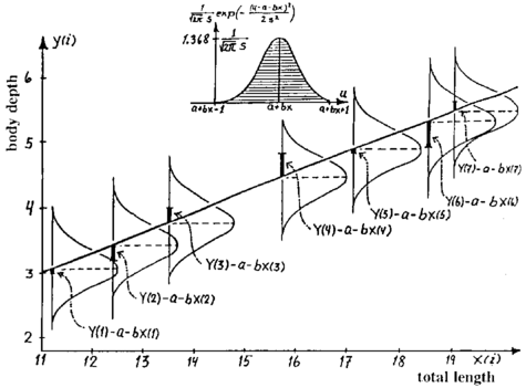
We can use this to rigorously test how well our linear regression fits the data. Sometimes we don’t need testing, but this is only when it’s so terrible that we need a better model…which is precisely the case we are in!
Dealing with Nonlinearity. Suppose we wanted to try to consider some nonlinear factor, like the exponential of the team’s weight in pounds…or something. We can transform the data before plugging it into the regression, so we get this new signal, and our linear regression becomes $y=a+bx+c\cdot\exp(w)$. This “preprocessing” allows the linear regression to be quite robust and useful, which is why its our first plan of attack against any problem.
Predictions
I made a number of predictions for the games scheduled on 21 June 2015, using a simple linear regression with the on-base percentage and slugging percentage as the input to generate the average number of runs per game. Lets see how this simple model performed…
Tigers vs Yankees
Prediction: .@tigers_former 5 vs .@Yankees 4
— Alex Nelson (@anelson_unfold) June 21, 2015The final score: Tigers 12, Yankees 4.
Rays vs Indians
Prediction: .@RaysBaseball 3 vs .@Indians 4.
— Alex Nelson (@anelson_unfold) June 21, 2015The final score was Rays 0, Indians 1.
Pirates vs Nationals
Prediction: .@Pirates 5 vs .@Nationals 3
— Alex Nelson (@anelson_unfold) June 21, 2015The final score: Pirates 2, Nationals 9.
Twins vs Cubs
— Alex Nelson (@anelson_unfold) June 21, 2015
The final score: Twins 0, Cubs 8.
Reflections on Results
Well, perhaps unsurprisingly, the predictions were bad. Although we predicted the Nationals would win against the Pirates, and Detroit would dominate the Yankees, we were comically wrong about the score. And we weren’t even close with the other games! The important question to ask is “Why?”
First, our data is far too coarse-grained. We tried making predictions about the results of a game using per-season data. One step forward would be to use data better suited to our problem. We will (next time) use Retrosheet’s data, which has play-by-play data for every game dating back to 1871.
Second, our model may be too simple. As noted earlier, there was the collinearity problem we never dealt with. But trying to figure out what combinations of data to use is rather taxing, especially when I don’t know a lot about the subject.
Next time we will model each play, and see if we can get better predictions.
References
- Neil Weinberg, How to evaluate a pitcher, sabermetrically and How to evaluate a hitter, sabermetrically.
- Charles Reid, “Are Batting Stats Useless?” Part 1, 2, 3. (The short answer appears to be “yes”)
- Phil Birnbaum, How to Find Raw Data chapter of A Guide to Sabermetric Research.
Changelog
- June 27, 2015: used table to display stats rather than raw REPL output, explained how to find the coefficients for a linear regression.