Insert in Red-Black Trees
by Alex Nelson, 24 October 2024
I wanted to talk about Stefan Kahrs’s delete method for persistent Red-Black trees (specifically, the “untyped” version). This requires reviewing inserting elements into a persistent Red-Black tree, and things snowballed very quickly. I had a huge blog post, which I decided to partition into two separate blog posts.
Before I begin, I should note that I am indebted to Tobias Nipkow’s book Functional Data Structures and Algorithms for his excellent discussion of functional data structures and proving properties about them using Isabelle/HOL. It’s really a delightful read, for anyone who wants to learn more about data structures in functional programming languages.
For brevity, I’m just going to drop the “persistent” adjective, and call things “Red-Black trees”.
Red-Black Trees
Red-Black trees are introduced by fiat as “some binary search tree” where each node has an “extra bit of information: its color (either Red or Black)”. Schematically, in Standard ML,
signature RED_BLACK_TREE = sig
  type value;
  val compare : value * value -> order;

  datatype Color = Red | Black;
  datatype Tree = Leaf
                | Node of Color * Tree * value * Tree;

  (* snip *)
end;
We will use the term “Red node” to refer to a node whose color is Red (and similarly “Black node” refers to a node whose color is Black).
Notation 1.
We will write:
- $\mathtt{Leaf}$ for
Leafin equations - $\langle\mathtt{Black},\ell,x,r\rangle$ for
Node(Black,l,x,r)in equations - $\langle\mathtt{Red},\ell,x,r\rangle$ for
Node(Red,l,x,r)in equations
Furthermore, if we want to discuss generic nodes in a binary tree, we
will write $\langle \ell,x,r\rangle$ to refer to them in equations.
(End of Notation 1)
Definition 2: Black height.
We will inductively define the Black Height of a Red-Black
tree as a non-negative integer $bh(t)\in\mathbb{N}_{0}$ defined by the
rules:
- $bh(\mathtt{Leaf}) = 0$
- $bh(\langle\mathtt{Black},\ell,x,r\rangle)=1+\max(bh(\ell),bh(r))$
- $bh(\langle\mathtt{Red},\ell,x,r\rangle)=\max(bh(\ell),bh(r))$
(End of Definition 2)
Further, a valid Red-Black tree satisfies four invariants:
- The root of the tree is Black.
- The empty tree is considered “Black” (so that the empty tree is a valid Red-Black tree).
- Red Invariant: No Red node has a Red child. An immediate corollary: no Red node has a Red parent.
- Black Invariant: The Black height of the left subtree is equal to the Black height of the right subtree; and, moreover, the left and right subtrees both satisfy the Black invariant.
When a Red-Black tree satisfies these four invariants, we will call it a Valid Red-Black tree.
Usually the discussion ends here, cryptically, without discussing the importance of the color. I want to discuss the importance of colors, but first we need to discuss a few notions and introduce a few terms.
Definition 3: Painting nodes.
Let $C$ be a color. We can define the operation of Painting
a Red-Black tree the color $C$ by cases as:
- Painting the empty tree produces the empty tree unchanged (since it does not have a color)
- Painting the node $\langle C’, \ell, x, r\rangle$ produces the node $\langle C, \ell, x, r\rangle$ with the desired color $C$.
(End of Definition 3)
Definition 4: (possibly) infrared trees.
We will call a Red-Black tree Infrared if its root node is
Red and the only possible Red invariant violation occurs at the root
node (i.e., the root node can have Red children).
We will call a Red-Black tree possibly-Infrared if painting
the tree Black produces a valid Red-Black tree. That is to say, it’s
either Infrared
or it violates only the “root is Black” invariant (but satisfies
both the Red and Black invariants)
or it’s Valid.
(End of Definition)
Chiral 2-4 Trees
So…what’s up with these colors?
We could make the analogy to “parasites” and “hosts”. A “parasite” feeds off of a host, but never off another parasite. A host has two sides for parasites. This is precisely the situation we have with Red nodes (“parasites”) and Black nodes (“hosts”).
A more visual way to think of Red-Black trees is as a sort of 2-4 tree (or a 2-3-4 Tree). This is not quite an isomorphism (a 3-node corresponds to two distinct Red-Black subtrees, which kills the dream of an isomorphism). We want an isomorphic description because then it’s just a “change of notation” describing “the same thing”.
We can recover an isomorphic description of Red-Black trees using Chiral 2-4 Trees where we have left-3-nodes and right-3-nodes.
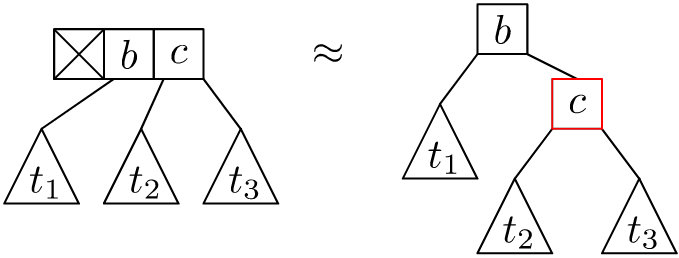
Specifically, we have right-3-nodes correspond to the following Red-Black tree:
The left-3-nodes correspond to the following Red-Black tree:
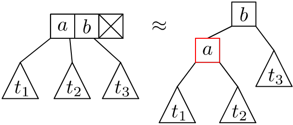
The “crossed out box” indicates a vacant spot for a Red child, and the “left”/”right” prefix indicates which spot the Red child lives.
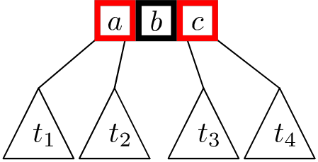
A 4-node then corresponds to a Black node whose children are both Red nodes.
Then:
- A Red node corresponds to left and right data elements in a node.
- A Black node corresponds to the “center element” of a node.
- The Black height of a Red-Black tree is equal to the height of the corresponding chiral 2-4 tree.
- The Red-invariant is automatically satisfied by the chiral 2-4 tree description.
- The Black-invariant asserts the chiral 2-4 tree is a “complete tree” (i.e., the leaves of the chiral 2-4 tree all live at “the same level”, in the sense that they all have the same depth).
You might hope therefore we could “import” the delete algorithm for 2-4 trees to apply to Red-Black trees (that was my hope, initially). Perhaps this could give us something nearly correct for a delete algorithm for Red-Black trees, but it is not the same as Kahrs’s delete algorithm. I discuss this further in the appendix to this article.
Remark: Historic motivation for Red-Black trees.
If you look at the original paper “A Dichromatic Framework for
Balanced Trees” by Guibas and Sedgewick on Red-Black trees, you will
find they explicitly were thinking of 2-4 trees (or “symmetric binary
B-tree” as they were called at the time) encoded as a binary
tree with nodes colored Black and Red. That is to say, we have
described the historic motivations for Red-Black trees, and not some
happy coincidence. This is because 2-4 trees are hard to reason about,
and hard to implement. Although Red-Black trees are still tricky
(hence this blog post!), they are far easier than 2-4 trees.
(End of Remark)
Drawing Red-Black Trees
I will take liberties when drawing Red-Black trees. Sometimes I will draw them as binary trees, with nodes being Red or Black boxes.
Othertimes I am going to draw Red-Black trees in a way resembling 2-4 trees,
since the Red nodes are “extensions” (“parasites”) to Black
nodes. For a Black node b with Red children a and b would be
drawn as:
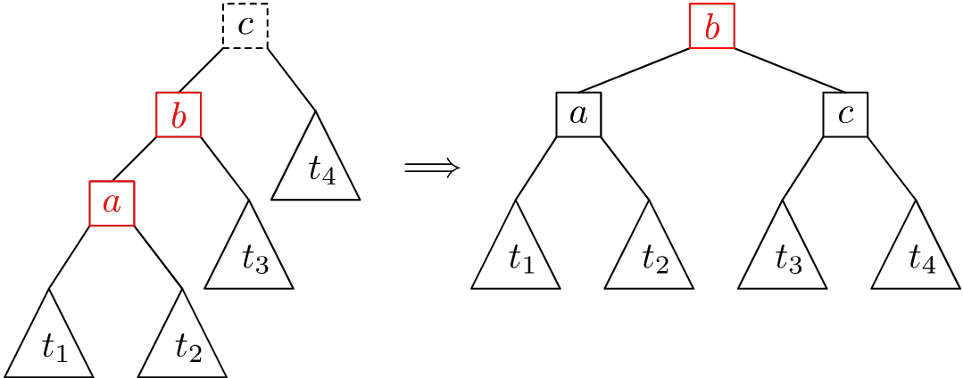
The edges between a Black node and Red children may be draw, or may be contracted to form a (chiral) 3-node or 4-node.
We will need to draw Red-Black trees as binary trees when we “pun” the usage of Red nodes to track “overflow” upon insertion, and “underflow” upon deletion, requiring rebalancing the Red-Black tree using tree rotations.
“Smart” constructors
Look, I’m lazy, so I will be abbreviating constructors for Red and Black nodes as:
(* "smart" constructors *)
fun R l x r = Node (Red, l, x, r);
fun B l x r = Node (Black, l, x, r);
Inserting Elements into a Red-Black Tree
The basic strategy, if we draw out a Red-Black tree, and try inserting a new value into the Red-Black tree, then the algorithm works as follows:
- Downward phase: We search to find where to place the new value.
- Then we insert the new value as a Red node.
- Upward phase: We rotate the parent Black node to restore the Red-Black invariants, producing a possibly-infrared Red-Black tree.
- We paint the root node of the resulting tree Black (to recover a valid Red-Black tree).
In Okasaki’s Functional Data Structures,
this is the approach he takes. In pidgin Standard ML, the “upward phase”
is handled by the balanceL and balanceR functions in:
(* right rotations to rebalance the tree *)
fun balanceL (Node (Red, Node (Red, t1, a, t2), b, t3)) c t4
    = R (B t1 a t2) b (B t3 c t4)
 | balanceL (Node (Red, t1, a, Node (Red, t2, b, t3))) c t4
    = R (B t1 a t2) b (B t3 c t4)
 | balanceL t1 a t2 = R t1 a t2;

(* left rotations to rebalance the tree *)
fun balanceR t1 a (Node (Red, t2, b, (Node (Red, t3, c, t4))))
    = R (B t1 a t2) b (B t3 c t4)
 | balanceR t1 a (Node (Red, (Node (Red, t2, b, t3)), c, t4))
    = R (B t1 a t2) b (B t3 c t4)
 | balanceR t1 a t2 = R t1 a t2;

fun insert x t =
  let
    fun ins Leaf = R Leaf x Leaf (* default case: insert a red node *)
     |  ins (Node(Black,l,a,r)) = (case compare(x,a) of
                                    LESS => balanceL (ins l) a r
                                  | EQUAL => B l a r
                                  | GREATER => balanceR l a (ins r))
     |  ins (Node(Red,l,a,r)) = (case compare(x,a) of
                                  LESS => balanceL (ins l) a r
                                | EQUAL => R l a r
                                | GRATER => balanceR l a (ins r));
  in
    (case (ins t) of
      (Node(_,l,a,r)) => B l a r
    | Leaf => B Leaf x Leaf) (* impossible *)
  end;
When the value x is not in the Red-Black tree, the insert
algorithm will insert it as a Red node. This possibly violates the
Red-invariant, which is why we need the balanceL and balanceR
functions.
The questions we should ask ourselves include: “Does this really work? If so, why?”
Well, we see that ins will look for a place to insert the new value x
into the tree t if possible.
- Case 1: If
xis not in the tree, it will eventually find a leaf, and replace this leaf with a red node containingx. - Case 2: If
xis in the tree, then nothing will be changed. (If you want to overwrite the value of the node, then you can change theEQUALcases in the definition ofinstoB l x randR l x rinstead.)
So far, we will have a binary search tree but not necessarily a valid Red-Black tree.
Then the balanceL and balanceR functions will rebuild the
Red-Black tree to ensure it is valid. After all, it is entirely
possible we inserted a Red child to a Red node.
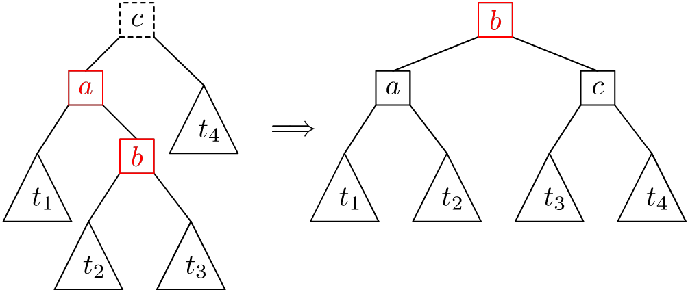
When we examine the circumstances when balanceL is called, we have
B l a r be a valid Red-Black tree. But we have balanceL (ins l) a r,
which means that ins l might have violated one of the invariants.
Well, what happens when we trying rebalancing the trees with
balanceL? We can draw diagrams for each of the three cases. (We can
do likewise for balanceR, it’s just a mirror image of these
diagrams, so the reader can test their understanding by drawing them.) The
first case:
Observe this is “just” a single right rotation, painting the nodes a
and c Black. Although this isn’t a valid Red-Black tree, it’s an
Infrared tree (and so if we painted it Black, it would be a valid
Red-Black tree).
The second case for balanceL can be drawn similarly:
Observe this describes a double-right rotation.
The “default” case for balanceL simply paints the root of the
subtree Red.
In all three cases, balanceL returns a Red-Black tree with a Red
root node. If this newly-Red node is the child of a Red node, then
we see that balanceL or balanceR will perform tree rotations and
paint nodes appropriately to fix things.
We can see then that balanceL and balanceR will return Infrared
trees which otherwise satisfy the Red-Black invariants.
But but but, what’s the deal with inserting Red nodes?
This is used to “flag” an overflow has occurred and the tree needs
rebalancing. Hence why the balanceL and balanceR functions perform
tree rotations (to restore balance) and then return an Infrared tree
(to indicate more rotations may be needed in the parent node to
restore balance recursively up the tree).
It’s not hard to prove the following theorem:
Theorem: Behaviour of balanceL.
If l is a possibly-Infrared tree and r is a valid Red-Black tree,
and if bh l = bh r, and if t' = balanceL l a r,
then t' is a possibly-Infrared tree without any Red-Red violations and bh
t' = 1 + bh l.
(End of Theorem)
The proof is straightforward by induction, but mildly tedious if done by hand.
A similar result may be proven describing balanceR.
Since ins will insert a new Red node, then recursively invoke
balanceL and balanceR, we see that rebuilding the tree will have
the mutated subtree have the same Black-height its untouched sibling
and more importantly satisfy the hypotheses of the aforementioned theorem.
This would rigorously prove that the result of ins produces a
possibly-Infrared tree. When we paint it Black, it becomes a valid
Red-Black tree (hence balanced).
Concluding Remarks
We should also prove that that height of a Red-Black tree of size $n\neq0$ is bounded by $2\log_{2}(n)$, but this is a straightforward proof found in many textbooks.
We should also implement a “lookup” function, but it’s the same as in any binary search tree.
I had hoped to discuss Kahrs’s delete algorithm, but found I needed to
discuss insert first to give some idea of what’s going on with the
rebalancing involved.