An Introduction to Neural Networks
by Alex Nelson, 1 August 2015
Abstract. We review neural networks, discussing the algorithms
behind the linear threshold perceptron, its failure at xor, the
forward-feeding neural network, and backpropagation. We make cursory
remarks about newfangled “recurrent neural networks”.
Contents
Introduction
We will use pseudocode throughout this article when discussing neural networks, it will be pidgin code.
Warning: We will use the term “perceptron” and “artificial neuron” interchangeably. Some texts make a distinction, we will not. (End of Warning)
Basic Perceptron
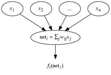
Inputs. A perceptron takes several binary inputs (or more generally, numeric inputs) x1, x2, …, and produces a single binary output.
The first step is to combine these inputs into a net input:
\begin{equation} \mathrm{net}_{i} = \sum_{j} w_{ij}x_{j}\tag{1} \end{equation}
where j runs over all inputs to the perceptron.
Activation Value. We then convert the net input into an “Activation Value”. We can write this as
\begin{equation} a_{i}(t) = F_{i}(a_{i}(t-1),\mathrm{net}_{i}(t))\tag{2} \end{equation}
for some function Fi. Observe we can make the activation value at time t depend on the activation value at the prior step. Usually, we just take ai(t) = neti(t).
Output Function. We then determine the output value by applying an “output function”: xi = fi(ai). We will take ai(t) = neti(t), so we will write xi = fi(neti).
Usually, some sigmoid function is chosen for f, like the logistic function or arc-tanh. But you can pick whatever function you want, just make sure it has a nice derivative (preferably one which can be written in terms of the original function, like the logistic function).
Summary for a single node. We can summarize the preceding comments for a single node using the following diagram (viewed from top-to-bottom):
Problems with XOR
Basic Idea.
Minsky and Papert’s Perceptrons (1969) studied a simple neural
network model called “single-layer neural networks”. They showed such a
network was incapable of simulating an xor gate.
Single-Layer Neural Network Model. Consider the Heaviside step function as our output function, i.e., H(x) = 1 if x is positive, and 0 otherwise. More generally, we can consider f(x) = H(x - θ) for some “threshold value” θ.
A single-layer neural network has precisely one layer. Since we want to consider a logic-gate, there would be one output — hence there is one node with two inputs, as doodled:
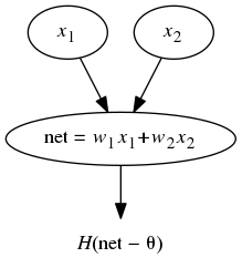
Classification of the Plane. This may be written in terms of the net-input: f(w1x1+w2x2). This amounts to dividing the (x1, x2) plane into two regions separated by the line θ = w1x1+w2x2.
Punchline.
The problem may now be stated thus: xor cannot be approximated by a
classifier which separates the plane by one straight line. This means we
cannot use a single-layer neural network model for approximating an
xor gate.
One solution is to say “Neural networks are useless”. This was a popular opinion since 1969 until very recently. The other would be to say “Single-layer networks are useless, we need more layers!” To the best of my knowledge, it was either the late ’80s or early ’90s when researchers decided having 3 layers was “good enough”. This is the “feedforward neural network”.
Remark (Solution). If you were wondering what sort of neural network actually solves this problem, a two-layer linear network will do it. We have the following graph representation:
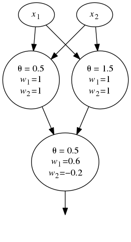
Or, if you’d prefer, as a single function
\begin{equation} f(x_{1}, x_{2}) =H(0.6H(x_{1}+x_{2}-0.5)-0.2H(x_{1}+x_{2}-1.5)-0.5) \end{equation}
The code for such a network is available in Clojure.
Backpropagation
An immediate question we should ask ourselves is “How on Earth could
anyone guess that as a solution to the XOR problem?!” It would be
disingenious for me to say “Well, I am oh so smart, and I just – zap! –
solved it.” Even if true, such a solution won’t scale well.
High-Level Description
Training. First, we need some training set to “teach” our network what to look for. More precisely: We have a set of P vector pairs (x1, y1), …, (xP, yP). These are examples of some mapping $\phi\colon\mathbb{R}^{N}\to\mathbb{R}^{M}$. We wish to approximate this as
\[\widehat{\mathbf{y}}=\widetilde{\phi}(\mathbf{x})\]based on our training data (the P vector-pairs).
The basic training algorithm may be summed up as:
- Apply the input vectors to the network, compute the output.
- Compare the actual output to the correct outputs, determine a measure of error.
- Determine which direction to adjust the weights in order to reduce error.
- Determine the amount to change each weight.
- Apply the corrections to the weights.
- Iterate steps 1 through 5 until the error is acceptable.
Although calling it “guess-and-check” may be a bit insincere, this describes the underlying mechanics of the so-called delta rule.
Step 1: Computing the Output. For a single output node, we have the following diagram describing N inputs to L hidden nodes to a single output:
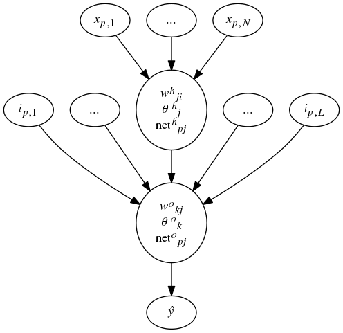
Given an input vector xp = (xp,1, …, xp,N)t, the input layer distributes the values to the hidden-layer. The net input to the jth hidden node is:
\begin{equation} \mathrm{net}^{h}_{pj} = \sum^{N}_{i=1} w^{h}_{ji}x_{p,i}+\theta^{h}_{j} \end{equation}
where whji is the weight on the conenction from the ith input layer, θ is the bias term. The superscript “h” reminds us this is for the hidden layer. We suppose the actiation of the node is its net input, the output for this node is then
\begin{equation} i_{pj} = f^{h}_{j}(\mathrm{net}^{h}_{pj}). \end{equation}
The equations for the output nodes are then:
\begin{align}
\mathrm{net}^{o}_{pk} &= \sum^{L}_{j=1}w^{o}_{kj}i_{pj} + \theta^{o}_{k}\\
\widehat{y}_{pk} &= f^{o}_{k}(\mathrm{net}^{o}_{pk})
\end{align}
where the o superscript reminds us this is the output layer.
Step 2: Determine Error. The error for a single input is
\begin{equation} \delta_{p,k} = y_{p,k} - \widehat{y}_{p,k} \end{equation}
where the subscript p keeps track of which training vector we’re working with, and the subscript k for which component of the vector we’re examining. We wish to minimize the error for all outputs, so we work with \begin{equation} E_{p} = \frac{1}{2} \sum^{M}_{k=1}\delta_{p,k}^{2} \end{equation} The one-half factor is for analytical calculations to simplify life later.
Steps 3 and 4: Determine direction and amount to change weights. This is a little bit involved mathematically. Really, we’re going to use a gradient-descent inspired approach, where we update the weights as \begin{equation} w^{o}_{kj}(t+1) = w^{o}_{kj}(t) + \Delta_{p}w^{o}_{kj}(t) = w^{o}_{kj}(t) - \eta\frac{\partial E_{p}}{\partial w^{o}_{kj}} \end{equation} where $\eta$ is called the learning-rate parameter, as per gradient descent. We use the chain-rule to find \begin{equation} \frac{\partial E_{p}}{\partial w^{o}_{kj}}= -(y_{p,k} - \widehat{y}_{p,k}) \frac{\partial f^{o}_{k}}{\partial(\mathrm{net}^{o}_{pk})} \frac{\partial(\mathrm{net}^{o}_{pk})}{\partial w^{o}_{kl}} \end{equation} hence \begin{equation} -\frac{\partial E_{p}}{\partial w^{o}_{kj}}=(y_{p,k} - \widehat{y}_{p,k}) f’^{o}_{k}(\mathrm{net}^{o}_{p,k})i_{p,j}. \end{equation} For the linear output unit, where $f^{o}_{k}(\mathrm{net}^{o}_{jk})=\mathrm{net}^{o}_{jk}$ we find $f’^{o}_{k}(\mathrm{net}^{o}_{jk})=1$. The logistic output unit, where \begin{equation} f^{o}_{k}(\mathrm{net}^{o}_{jk}) = [1 + \exp(-\mathrm{net}^{o}_{jk})]^{-1} \end{equation} we find \begin{equation} f’^{o}_{k}=f^{o}_{k}(1-f^{o}_{k}). \end{equation} Generally, we would like $f$ to be such that its derivative is sufficiently nice…and would minimize the amount of recalculations.
Observe this updates the weight for the output layer, we must update the weights for the hidden layer too!
Updating weights for Hidden Layer. We use the chain rule again, computing \begin{equation} \frac{\partial E_{p}}{\partial w^{h}_{ji}}= -\sum_{k}(y_{p,k} - \widehat{y}_{p,k}) \frac{\partial \widehat{y}_{p,k}}{\partial(\mathrm{net}^{o}_{pk})} \frac{\partial(\mathrm{net}^{o}_{pk})}{\partial i_{pj}} \frac{\partial i_{pj}}{\partial(\mathrm{net}^{h}_{pj})} \frac{\partial(\mathrm{net}^{h}_{pj})}{\partial w^{h}_{ji}} \end{equation} We find after some algebra \begin{equation} \Delta_{p}w^{h}_{ji} = \eta x_{p,i}\delta^{h}_{p,j} \end{equation} where \begin{equation} \delta^{h}_{p,j} = f’^{h}_{j}(\mathrm{net}^{h}_{p,j})\sum_{k}\delta^{o}_{p,k}w^{o}_{kj}. \end{equation} We have to propagate the error through all the hidden layers, which just amounts to iterating this procedure. There are a lot of subtle problems with deep networks (recall, a neural network is ‘deep’ if it has more than one hidden layer). We won’t worry about them here, we’re working with a vanilla network.
Momentum
One last remark, Freeman and Skapura discuss adding an extra term to the delta rule: \begin{equation} w^{o}_{k,j}(t+1) = w^{o}_{k,j}(t) + \Delta_{p}w^{o}_{k,j}(t) + \alpha\Delta_{p}w^{o}_{k,j}(t-1) \end{equation} where $0\lt\alpha\lt1$ is called the “Momentum” and brings a contribution of $\Delta w$ from the previous iteration. It is optional, usually it speeds up convergence, but I have not seen many people discussing this…so I’m guessing it fell out of favor for a reason.
Algorithm
In pidgin C/Java/D/blub code, we have the following data structure for the layer
struct Layer {
    double outputs[];       /* outputs for the given inputs */
    double weights[][];     /* the connection array */
    double errors[];        /* error terms for the layer */
    double last_delta[][];  /* previous delta terms for the layer */
};
We can thus construct a network using this:
struct Network {
    Layer *input_units;   /* The input layer */
    Layer *output_units;  /* Output units */
    Layer layers[];       /* dynamically sized layers */
    double alpha;         /* momentum term */
    double eta;           /* learning rate parameter */
};
Forward Propagation Routines
We need a helper function to set the inputs for a network. I don’t want to get caught up in the minutae of pointers, so if you’re concerned about it…just bear with me.
void setInputs(Network *network, double input[]) {
    double **network_inputs = &(network->input_units->outputs);
    /* copy the input to the neural net's input layer */
    for (int i=0; i<length(input); i++) {
        network_inputs[i] = input[i];
    }
}
We can easily propagate a single layer now. We assume that the output
function f is abstracted out into its own outputFunction().
/* for us, sigmoid */
double outputFunction(double x) {
    return 1.0/(1.0 + exp(-x));
}

void propagateLayer(Layer *lower, Layer *upper) {
    int i,j; /* iteration counts */
    double sum;
    double **connects;
    double **inputs = &(lower->outputs);  /* locate the lower layer */
    double **current = &(upper->outputs); /* locate the upper layer */

    /* for each node in the output layer */
    for(i=0; i<length(current); i++) {
        /* reset the accumulator */
        sum = 0;
        /* locate the weight array */
        connects = &(upper->weights[i]);
        /* for each node in the input */
        for (j=0; j<length(inputs); j++) {
            /* accumulate the products */
            sum = sum + inputs[j]*connects[j];
        }
        current[i] = outputFunction(sum);
    }
}
Now we can work with the entire network.
void propagateForward(Network *network) {
    Layer *lower;
    Layer *upper;
    int i;

    /* for each layers */
    for(i = 0; i<length(network->layers); i++) {
        /* locate the lower and upper layer */
        lower = &(network->layers[i]);
        upper = &(network->layers[i+1]);
        /* propagate forward */
        propagateLayer(lower,upper);
    }
}
The last thing we would want to do would be copy the outputs into an array.
void getOutputs(Network *network, double outputs[]) {
    double **network_outputs = &(network->output_units->outputs);
    int i;

    /* copy the array over, element by element */
    for(i=0; i<length(network_outputs); i++) {
        outputs[i] = network_outputs[i];
    }
}
Error Propagation Routines
First, we need our helper function…the derivative of the sigmoid. You can swap this for whatever you are using, I just want to include it for completeness.
double derivativeOutputFunction(double y) {
    return y*(1.0-y);
}
Great, now we compute the values of $\delta^{o}_{p,k}$ for the output layer.
void computeOutputError(Network *network, double target[]) {
    double **errors = &(network->output_units->errors);
    double **outputs = &(network->output_units->outputs);
    int i;

    for(i=0; i<length(outputs); i++) {
        errors[i] = (target[i]-outputs[i])*derivativeOutputFunction(outputs[i]);
    }
}
Now we write a routine to backpropagate to the hidden layer.
/* backpropagate errors from an upper layer to a lower layer */
void backpropagateError(Layer *upper, Layer *lower) {
    double **senders;   /* source errorrs */
    double **receivers; /* receiving errors */
    double **connects;  /* pointer to weight arrays */
    double unit;        /* unit output value */
    int i,j;

    senders = &(upper->errors);
    receivers = &(lower->errors);

    for(i=0; i<length(receivers); i++) {
        /* initialize the accumulator */
        receivers[i] = 0;
        /* loop through the sending units */
        for(j=0; j<length(senders); j++) {
            /* get the weights for the given node */
            connects = &(upper->weights[j]);
            receivers[i] = receivers[i] + senders[j]*connects[i];
        }
        /* get the unit output */
        unit = lower->outputs[i];
        /* set the receiver */
        receivers[i] = receivers[i] * derivativeOutputFunction(unit);
    }
}
We need to lastly update the weights for the network. We’ll use the momentum and whatnot, iterating through all the layers.
void adjustWeights(Network *network) {
    Layer *current;
    double **inputs;
    double **units;
    double **weights;
    double **delta;
    double **error;
    int i, j, k;xs

    /* starting at first computed layer */
    for(i=1; i<length(network->layers); i++) {
        current = network->layers[i];
        units = &(network->layers[i]->outputs);
        inputs = &(network->layers[i-1]->outputs);

        /* for each unit in the layer */
        for(j=0; j<length(units); j++) {
            weights = &(current->weights[j]); /* find input connections */
            delta = &(current->delta[j]); /* find last delta */
            error = &(network->layers[i]->errors);

            /* update the weights connecting that unit */
            for(k=0; k<length(weights); k++) {
                weights[k] = weights[k] + (inputs[k]*(network->eta)*error[k]); /* generalized delta */
                weights[k] = weights[k] + ((network->alpha)*delta[k]); /* momentum term */
            }
        }
    }
}
Big Red Button!
We now have two basic methods, one to train the network, the other to predict.
double[] predict(Network *trained_network, double input[]) {
    size_t output_length = length(trained_network->output_units->outputs);
    double *outputs = new double[output_length];

    setInputs(trained_network, input);
    propagateForward(trained_network);
    getOutputs(trained_network, outputs);

    return outputs;
}
We have a helper function to compute the error of the network on some
given list of training inputs and targets. I assume the indices for the
double arrays are of the form inputs[p] gives the pth
training vector’s input (what we previously called
_x_p), and inputs[p][k] gives its kth
component.
double error(Network *network, double inputs[][], double targets[][]) {
    int i, j;
    double outputs[];
    double err = 0.0;
    double term;
    for(i=0; i<length(inputs); i++) {
        outputs = predict(network, inputs[i]);
        for(j=0; j<length(outputs); j++) {
            double term = targets[i][j]-outputs[j];
            error = error + term*term;
        }
    }
    return 0.5*err;
}
The training requires an array of input vectors, an array of output vectors, some tolerance (cutoff for the error to be “good enough”), and a network to train.
void train(Network *network, double inputs[][], double targets[][], double tol) {
    int i, j;
    do {
        /* foreach training pair, train the network */
        for(i=0; i<length(inputs); i++) {
            setInputs(network, inputs[i]);
            propagateForward(network);

            /* determine the errors */
            computeOutputError(network, targets[i]);

            /* update the error values on all the layers */
            for(j=length(network->layers)-1; j>0; j--) {
                backpropagateError(network->layers[j], network->layers[j-1]);
            }

            /* modify the network */
            adjustWeights(network);
        }
    /* until error is good enough */
    } while (error(network, inputs, targets)>tol);
}
Concluding Remarks
Training a neural network is usually very slow, and the deeper the network…the slower it goes. There are ways to speed it up, like picking features that “contribute the most” (in the sense of maximizes entropy) or making a “stochastic gradient descent”-inspired training algorithm.
One last comment, since I promised earlier, about recurrent neural networks. The textbook definition is just a neural network with a nontrivial topology. What, e.g., Google means by an RNN is that we have several networks in parallel that have distinct segments of the input vector. We take the hidden layer from the first network, and use it as if it were part of the input layer for the second network (in the sense that it feeds into the second network’s hidden layer). We can iterate this process (taking the hidden layer from the second network, and using it as input into the third, and so on). Apparently this produces amazing results.
References
- Amanda Gefter, The Man Who Tried to Redeem the World with Logic. A well written article about the man who, basically, invented Neural networks from scratch.
Theory
- John Hertz, Anders Krogh, and Richard G. Palmer, Introduction to the Theory of Neural Computation. Addison-Wesley, 1991.
Algorithms
- James A. Freeman and David M. Skapura, Neural Networks: Algorithms, Applications, and Programming Techniques. Addison-Wesley, 1991.
- Michael Nielsen, Neural Networks and Deep Learning. A free, and quite good, ebook on the subject.